 (1)
(1)
The form of the partition functions will be shown to be different depending on whether the particles are distinguishable or not. Furthermore, if the particles are boson or fermion, the form of the partition functions also differ. As a consequence, the distribution of particles will also differ. These are the topics we will discuss in this lecture.
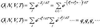
(1)
| We can do this: | |
| if Hamiltonian can be written as a sum of independent terms | |
| if particles are distinguishable! |
If the energy of all particles are the same, the above equation becomes
 | for Distinguishable Particles | (2) |
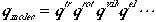
As we have seen in the discussion above, the Hamiltonian can be separated into a sum of various degrees of freedom, and therefore, we can write
 (3)
(3)
Tremendous simplification in calculating partition functions is achieve by using Eqns. (1) and (3); we have reduced an N-body problem to one-body problem, and further reduced to individual degrees of freedom of one particle.
The total energy of the system and the partition function are
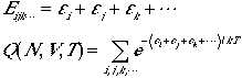 (4)
(4)
Since the particles are indistinguishable, we can not do what we did
in Eqn. (1), i.e. to sum the indices individually.
Consider the following, where all indices except one is the same,
 (5)
(5)
Since the indices are just dummy the position of
ei is not important. If we sum over all states,
we overcount the sum by N.
Consider another case, where all indeces are different, such that
 (6)
(6)
The N! states obtained by permuting N different subscripts
are identical, and occur only once in the summation. But, in general,
it occurs N! times.
Reality lies somewhere between the two extreme above. However, if we consider that there are many many more states available to the particles, then we have the latter situation.
The number of quantum states available to the system for energy less than e is of order O(1030), if we use a particle-in-a-box (3D) approximation; mass = 10-22g in a 10 cm cube at 300 K. This shows that the available quantum states are much larger than the number of the particles in the system! Hence, molecules can choose quantum states of choice, and the summation in Eqn. (4) should have different indices occupied.
Then, by summing over all states and then divide by N!, and we arrive at.
| Approximation to Eqn. (4) for indistinguishable particles | ||
|---|---|---|
 |
for # of available quantum states >> N | (7) |
Indistinguishability of the particles is incorporated into
the equation with the condition that the number of available quantum
states to be much larger than the number of particles.
This is said to obey Boltzmann statistics.
The condition for Boltzmann statistics is to have large mass,
high temperature and low
density. Such condition is the classical mechanics limit.
The total energy of the N-body system is
Therefore, the average energy of a particle is
 (8)
(8)
which leads to the probability that a molecule is in the jth
state is
 (9)
(9)
It follows that the fluctuations in molecular energies can be shown
and the fluctuations in energies are of order e.
A sharp probability distribution seen in previous sections are
many-body effect!
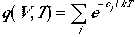
Consider a grand canonical ensemble. Let Ej(N,V) be the available states for N molecule system, and ek be the molecular quantum states. The energy of the system is given by

and also

Canonical partition function, Q(N,V,T) can be written as
 (10)
(10)
The asterisk in the summation denotes for the restriction
that the total number being fixed at N.
It turns out that this restriction is mathematically awkward in canonical ensemble. By using a grand canonical ensemble, the evaluation of the partition functions are easier. We write the grand canonical partition function as
 .
.
This can be written as

by defining l =
ebm. Then, we arrive at
Since we are summing over all values of N, each nk
ranges over all possible values, we can write
It can, then, be rewritten as
and arrive at a general expression
 | (11) |
Now for a fermion system, the occupation, nk can only be 0 or 1 due to Pauli exclusion principle. Therefore, n1max = 1, and arrive at:
 | Fermi-Dirac Statistics | (12) |
For a boson system, there is no restriction in occupation therefore, nk extends to infinity, and we have
However, if we use the following math. identity,
we can arrive at:
 | Bose-Einstein Statistics | (13) |
Since average N can be written as,
It follows that
Therefore, the average number of particles in the kth
quantum state is given by

which is in analogy with Eqn. (9) above.
Then the average energy in quantum statistics is given by

We can also derive expression for the following.

Next, we will look at ideal monatomic and diatomic gases.