Chapter 3. Quantum Mechanics in a Nutshell

Schrödinger Equation

Time-independent Schrödinger equation is

[- \frac{ℏ^{2}}{2 m} \nabla_{x}^{2} + V (x)] Ψ (x) = E Ψ (x)

where i is the √(-1), ℏ is Planck's constant divided by 2π, m is the mass, ∇² is the second derivative operator with respect to coordinate (d²/dx² in this case), and V(x) is the potential energy operator. Ψ(x) and E are, respectively, wave function and energy of the system.

We are going to look at details of how we solve Schrödinger equation for certain systems, including chemical systems that we are famililar with, such as reaction energies and transition state structure and activation energy.

The form of Schrödinger equation does not change, but different system has different potential energy (or shape of potential energy) for which we model the physical system. So, in one sense, we seek solutions, meaning that we look for Ψ(x) that satisfy the equation, then at the same time, we can learn about the energy of the state of the system.

For a larger system, multiparticle cases, we must think of additional strategy, but it would be simple enough for relatively simple systems. For electronic structure of molecules, we must go beyond the simple approach and incurr another level of strategy.

Here is what Schrödinger might have done for derivation of the equation.

+ A posteriori Derivation

We start with De Broglie's equation for particle wave length, λ,

λ = \frac{h}{p}

where h is Planck's constant and p is the particle momentum. From classical mechanics of wave, the wave amplitude, Ψ is given by following equation,

\nabla^{2} Ψ = - k^{2} Ψ

where ∇ = d/dx and k = 2π/λ is the wave vector. By substituting above into Eqn. C1,

\nabla^{2} Ψ = - {(\frac{2 π p}{h})}^{2} Ψ = - \frac{4 π^{2} p^{2}}{h^{2}} Ψ

Since E = T + V, and

$E = \frac{1}{2} m v^{2} + V$	C4
$m v^{2} = 2 (E - V)$	C5

By substituting Eqn. C5 into Eqn. C3, with understanding that p² = m(mv²),

\nabla^{2} Ψ = - \frac{4 π^{2} m (2 (E - V))}{h^{2}} Ψ

and rearrange Eqn. C6 to obtain

- \frac{ℏ^{2}}{2 m} \nabla^{2} Ψ + V Ψ = E Ψ

where ℏ = h/2π.

Quantum Mechanical Postulates

Before we move on to solving Schrödinger equation, we need to understand that quantum mechanics is based upon several postulates. Even though, these are postulates, for application to chemistry these have not deviated from the experimental findings.

Here we list six postulates:

1) For any state of a system, there is a wave function Ψ, that depends on the coordinates of the system and time, describes the system completely.

Ψ = Ψ (x_{1}, x_{2}, x_{3}, \dots, x_{N}, t)

where N is the maximum number of coordinates in the system.

In general the wave function can be complex numbers. The wave function is the key in understanding the quantum system. Much of studies applies quantum mechanics devoted to solve the wave function. By itself, the wave function does not have physical meaning.

2) For every observable quantity, there exists a corresponding linear Hermitian operator. We will look at this more closely in the next section.

3) The state function Ψ is given as a solution to the Schrödinger equation

\hat{H} Ψ = E Ψ

Schrödinger equation itself is a postulate. This is the equation that gives meaning to the wave function. In the case of the observable, energy, the physical system is described by Hamiltonian operator,

\hat{H}

, which is

\hat{H} = \hat{T} + \hat{V}

where

\hat{T}

is the kinetic energy operator and

\hat{V}

is the potential energy operator.

4) The state function Ψ also satisfies

i ℏ \frac{\partial Ψ}{\partial t} = \hat{H} Ψ

This is called time-dependent Schrödinger equation, describing time evolution of the wave function when no one is looking. The dynamics of quantum system is described by the time-dependent Schrödinger equation.

5) The square of the state function, |Ψ(x,t)|²dτ, gives probability density of the particle in the system, with the dτ describes the volume element. This postulate is due to Max Born.

6) The average quantity in quantum mechanics for a given operator is called expectation value, which is

〈 \hat{O} 〉 = \frac{\int Ψ^{*} \hat{O} Ψ d τ}{\int Ψ^{*} Ψ d τ} = \frac{〈 Ψ | \hat{O} | Ψ 〉}{〈 Ψ | Ψ 〉}

Eigenvalue Equation: Schrödinger Equation

The time-independent Schrödinger equation, is given as eigenvalue equation. You notice that Hamiltonian operator operated on the wave function gives energy E and the same wave function back. One way to understand what Schrödinger equation tells is to consider physical meaning of the equation. Regardless of where the equation comes from (in fact, one can not derive Schrödinger equation--Schrödinger fudged it somehow during the Christmas holiday in the Tyrollean Mountains), it tells you that Hamiltonian operator describes the physics of the system. It contains operators for kinetic and potential energy. As was the case in the classical mechanics, the kinetic energy plus the potential energy in the phase space gives total energy of the system. Also as in the classical mechanics, the total energy a constant of motion, meaning that the total energy of the system is a conserved quantity.

Another way to look at this equation is that the total energy is given by transforming the operator into coordinate independent quantity, such as energy via the wave function. The transformation of the kind, $\hat{H} \to E$ , is for Schrödinger equation. Therefore, you should ask yourself a question, "Given the kinetic energy and the between the particles, what wave function gives me the energy?" The answer to this question gives the solution to Schrödinger equation. By the way, as we mentioned before, the force between particles is given by $F = - \frac{\partial V (x)}{\partial x}$ . In atoms and molecules, the forces between electrons and nuclei are based on electromagnetic forces, in particular Coulomb attractions and repulsions.

Let's look at properties necessary to construct mathematical structure of quantum mechanics next.

Conditions on Ψ to be well-behaved

1) Single-valued so that the probability is unambiguously normalizable.
2) Continuous
3) Nowhere infinite
4) Piecewise continuous of the first derivatives
5) Commutation with constant
6) Square-integrable

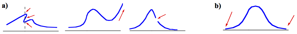
Figure 1. a) Examples of bad wave function, b) good wave function.

Examples of bad and good wave functions look like, are shown in Figure 1. The first panel of a) is not single-valued, thus it is not even a function. The second panel of a) has one side tended toward infinity. The third has a break 2) and the first derivatives also don't seem to match 4). Figure 1b is an example of good wave function that satisfies all conditions.

The last one, square integrability, hits the core of quantum mechanics. First, it means that the integral of the probability density must be finite. This is so that to the wave function is normalizable. It makes perfect sense when you consider a physical system where the particle in the system must exist somewhere in the system! This is expressed mathematically, in the denominator of Eqn. 5,

\int Ψ^{*} Ψ d τ = c

where Ψ^* is the complex conjugate of Ψ.

The wave function can be complex,

Ψ = Ψ_{r e} + i Ψ_{i m}

where Ψ_re is the real part of the total wave function, i is square-root of negative 1, and Ψ_im is the imaginary part. The complex conjugate is constructed by changing the sign on the imaginary part,

Ψ = Ψ_{r e} - i Ψ_{i m}

Therefore when we say square-integrate the wave function, we mean to incorporate the sign change in the integration. Thusly,

〈 Ψ | Ψ 〉 = \int (Ψ_{r e} - i Ψ_{i m}) (Ψ_{r e} + i Ψ_{i m}) d τ = \int (Ψ_{r e}^{2} + Ψ_{i m}^{2}) d τ

The right-hand side of Eqn. 7 must be positive value. If we take Ψ is taken as unnormalized wave function we can obtain normalized function, Ψ' = AΨ, where A is the normalization factor. The square integrating the normalized wave function is forced to be one.

$\int Ψ'^{*} Ψ' d τ = 1$	8
$A^{2} \int Ψ^{*} Ψ d τ = 1$	9
$A^{2} c = 1$	10
$A = {(\frac{1}{c})}^{1 / 2}$	11

In going from Eqn. 9 to Eqn. 10, Eq. 4 is used. Therefore, the normalized wave fucntion is

Ψ' = {(\frac{1}{c})}^{1 / 2} Ψ

Operators

The observable quantities in quantum mechanics is expressed in terms of operators. Operator is used in eigenvalue equation (Eqn. 3). When operated on eigenfunction, Ψ, the operator is transformed into eigenvalue. In Eqn. 3, Hamiltonian operator,

\hat{H}

, is transformed into energy, E.

For us, we need mostly two operators that are important in understanding chemistry, and these are: momentum operator and coordinate operators. These constitute the component of Hamiltonian operator as well as some of the spectroscopic quantities, such as dipole moment operator.

Momentum operator

The momentum operator is given in one dimension (x coordinate) is

{\hat{p}}_{x} = - i ℏ \frac{\partial}{\partial x}

where ℏ is Planck's constant divided by 2π. So, if you have

Ψ = A e^{i k x}

as a wave function, its momentum is, then

\hat{p} Ψ = ℏ k A e^{i k x} = ℏ k Ψ

Therefore, the momentum p = ℏ k.

Coordinate operator

The coordinate operator is a multiplicative operator of coordinate, say x. So,

\hat{x} Ψ = x Ψ

This operator is used in spectroscopy often. The dipole moemnt operator is given as

\hat{d} = q \hat{x}

We can use Eqn. 16 in the expectation value of the dipole operator which is the dipole moment.

〈 Ψ | \hat{d} | Ψ 〉 = q 〈 Ψ | \hat{x} | Ψ 〉

Function operator

A function f(x) is operated on Ψ. Again, we can express in terms of expectation value of, for example, of potential energy of diatomic molecule,

V (x) = D_{e} {(1 - e^{- a (x - x_{e q})})}^{2}

is called Morse function where D_e is the dissociation energy and a is a constant related to the force constant.

〈 Ψ | \hat{V} (x) | Ψ 〉

can be described as part of matrix elements to calculate vibrational energies of diatomic molecule represented by Morse function.

Hamiltonian operator

Hamiltonian operator is to calculate the energy of the system. Since the total energy is expressed classically as

H = T + V

where T is the kinetic energy and V is the potential energy. The quantum mechanical expression in terms of operator is Hamiltonian operator. We saw this already in Eqn. 1, but let me reiterate here, in terms of operator.

\hat{H} = \hat{T} + \hat{V} = - \frac{ℏ^{2}}{2 m} \frac{\partial^{2}}{\partial w^{2}} + V (w)

where m is the mass. In general, the number of coordinates, w, is 3 (or 4, if one includes spin) for a given particle, therefore, the partial derivative is used in the kinetic energy operator.

Commutation relation

When two coordinate operators, say x and y, are used to operate on a wave function, the order of the operator doesn't matter in obtaining eigenvalues.

$\hat{x} \hat{y} Ψ = x y Ψ$	21
$\hat{y} \hat{x} Ψ = y x Ψ = x y Ψ$	22

since x and y are just numbers. But when derivative operator is used, the order matters.

\hat{d} \hat{x} Ψ \neq \hat{x} \hat{d} Ψ

where

\hat{d} = \frac{d}{d x}

. For example,

\hat{d} \hat{x} Ψ = x Ψ^{'} + Ψ \neq \hat{x} \hat{d} Ψ = x Ψ^{'}

The operators

\hat{x}

and

\hat{d}

are said to be not commutative. And if they are equal, then they are said to be commutative.

$\hat{A} \hat{B} - \hat{B} \hat{A} = 0$	Commuting Operators	25
$\hat{A} \hat{B} - \hat{B} \hat{A} \neq 0$	Noncommuting Operators	26

When two operators commute, simultaneous measurements corresponding to the eigenvalues of the two operators are possible. On the other hand, the two operators don't commute, one can not measure eigenvalues simultaneously.

The commutation relation is expressed with a square bracket, as

[\hat{A}, \hat{B}] = \hat{A} \hat{B} - \hat{B} \hat{A}

For example, again,

\hat{x}

and

\hat{p}

[\hat{x}, \hat{p}] Ψ = i ℏ (- x \frac{d}{d x} + \frac{d}{d x} x) Ψ = i ℏ (- x \frac{d Ψ}{d x} + x \frac{d Ψ}{d x} + Ψ) = i ℏ Ψ

So,

[\hat{x}, \hat{p}] = i ℏ

This is one of the major result obtained by Heisenberg.

Uncertainty principle

Using the result, Eqn. 29, Heisenberg was able to deduce the one of the most important concepts in quantum mechanics, uncertainty principle, which states that the product of the errors associated with the measurements of coordinate and speed must be greater than or equal to ℏ/2.

δ x δ p \geq \frac{ℏ}{2}

+ Uncertainty Derivation

The variance, square of error, in x and p are

${(δ x)}^{2} = 〈 {(\hat{x} - 〈 x 〉)}^{2} 〉 = \int Ψ^{*} {(\hat{x} - 〈 x 〉)}^{2} Ψ d x$	C1
${(δ p)}^{2} = 〈 {(\hat{p} - 〈 p 〉)}^{2} 〉 = \int Ψ^{*} {(\hat{p} - 〈 x 〉)}^{2} Ψ d x$	C2

Eqns. C1 and C2 along with Eqn. 29 are used to derive the uncertainty relation. Here < > indicates the average value. The deviation δx is root-mean-square deviation in x from the average value of x, i.e. <x>, and similar language can be used for p. So, the deviation is a spread of the quantity under consideration. The relation tells us that when the two systems are prepared identically, and try to measure position and speed simultaneously in each system, you would not obtain the same measurement twice.

If we define Ψ_x and Ψ_p to be

$Ψ_{x} = (\hat{x} - 〈 x 〉) Ψ$	C3
$Ψ_{p} = (\hat{p} - 〈 p 〉) Ψ$	C4

Then the variance of momentum, δp, can be calculated as

$〈 Ψ_{p} \| Ψ_{p} 〉 = \int Ψ_{p}^{} Ψ_{p} d x = \int {[(\hat{p} - 〈 p 〉) Ψ]}^{} (\hat{p} - 〈 p 〉) Ψ d x$	C5
$= \int Ψ^{*} {(\hat{p} - 〈 p 〉)}^{2} Ψ d x = {(δ p)}^{2}$	C6

Similarly,

〈 Ψ_{x} | Ψ_{x} 〉 = {(δ x)}^{2}

Now, what we want to do is to create a condition for inequality of certain type to exist. Let us first make a linear combination of Ψ_x and Ψ_p,

Ψ = Ψ_{x} - i k Ψ_{p}

When we square integrate the wave function C8, it should give a positive number, if the wave function is well-behaved.

〈 Ψ | Ψ 〉 \geq 0

Let us expand on this.

〈 Ψ | Ψ 〉 = {\int (Ψ_{x} - i k Ψ_{p})}^{*} (Ψ_{x} - i k Ψ_{p}) d x \geq 0

C10

$= \int (Ψ_{x} + i k Ψ_{p}) (Ψ_{x} - i k Ψ_{p}) d x$	C11
$= \int [Ψ_{x}^{2} - i k (Ψ_{x}^{} Ψ_{p} - Ψ_{p}^{} Ψ_{x}) + k^{2} Ψ_{p}^{2}] d x$	C12

Since the terms in the parenthesis of Eqn. C12 is a commutator between x and p due to the fact that <x> and <p> are just numbers, they can be taken out of the integral, leaving operators of x and p. Hence,

〈 Ψ | Ψ 〉 = \int [Ψ_{x}^{2} - i k [\hat{x}, \hat{p}] + k^{2} Ψ_{p}^{2}] d x = \int [{(δ x)}^{2} + k ℏ + k^{2} {(δ p)}^{2}] d x \geq 0

C13

In the last step, we used Eqn. 29. Then, in order for the integral to be positive, the quadratic equation of k must also be positive.

{(δ x)}^{2} + k ℏ + k^{2} {(δ p)}^{2} \geq 0

C14

Furthermore, for any value of k to be applicable, the solution to have unique positive real solution in the following.

\frac{- ℏ \pm {(ℏ^{2} - 4 {(δ p)}^{2} {(δ x)}^{2})}^{1 / 2}}{2 Ψ_{p}^{2}}

C15

The positive real unique solution is only obtained through the square root term, discriminant D, to have negative value, that is

D = ℏ^{2} - 4 {(δ p)}^{2} {(δ x)}^{2} \leq 0

C16

Eqn. C16 immediately leads to

\frac{ℏ^{2}}{4} \leq {(δ p)}^{2} {(δ x)}^{2}

C17

Hence, Eqn. 30 is obtained.

Coordinate and momentum are conjugate variables and they do not commute. Energy and time are also conjugate variables, thus life time of the state and energy are not simultaneously measurable. Fourier transformation connects one variable to the other. The time domain signals in NMR can be Fourier transformed into frequency domain to obtain NMR spectra.

In explaining the relation, Heisenberg used one of the greatest gedanken experiment. In this thought experiment is to show how simple act of observation can change the trajectory of quantum particle because of photon can interact with the quatnum particle.

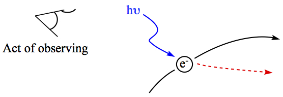
Figure 2. Heisenberg's gedanken experiment on trajectory of electron

Act of looking requires turning a light on. In order to make sharper image of the quantum particle, one must send higher frequency light to the quantum particle. The image (or position) of the particle is now sharp, but because high frequency light would interact with the particle strongly and change the momentum of the particle enough to blurr the velocity of the particle. Opposite can also happen where in order to sharpen the velocity, the position is blurred with low frequency light.

Fundamentally, in the quantum regime, particle trajectory in the sense of classical mechanics lose its meaning. Act of merely looking at particles influence the behavior of quantum particles.