Chapter 5. Many Electron Atoms

Variational Method

Up to this point, all problems we have examined are analytically solved. In many electron atoms and molecules, it is no longer possible to solve Schrödinger equation analytically. We must then seek solution to Schrödinger equation in approximate manner. If possible, approximation we use can be obtained through either systematic manner or we know the error associated with the approximation. We present variational method and perturbation theory for this purpose.

Ritz Variational Principle

Let us denote the ground state energy to be E₀ for which we don't have explicit solution of Schrödinger equation. However, we have

$$H{\psi }_n=E_n{\psi }_n$$

1

So, the wave function of state n forms an orthonormal set, $\langle {\psi }_n|{\psi }_m\rangle ={\delta }_{nm}$. Since the wave function is complete set, we can form a linear combination, such that

$$\varphi ={\displaystyle \sum _m{a}_m{\psi }_m}$$

2

and

$${{\displaystyle \sum _m\left|a_m\right|}}^2=1$$

3

If we substitute Eqn. 2 into the expectation value of E,

$$\langle E\rangle =\frac{\langle \varphi |\widehat{H}|\varphi \rangle }{\langle \varphi |\varphi \rangle }$$

4

we get,

$$\langle \varphi |\widehat{H}|\varphi \rangle ={\displaystyle \sum _{m,n}{a}_n\langle {\psi }_n|\widehat{H}|{\psi }_m\rangle }{a}_m={\displaystyle \sum _{m,n}{a}_n}\langle {\psi }_n|E_m|{\psi }_m\rangle a_m={\displaystyle \sum _{m,n}{a}_n}{E}_m\langle {\psi }_n|{\psi }_m\rangle a_m={\displaystyle \sum _n{a}_n^2}{E}_n$$

5

The denominator is equal to one due to Eqn. 3 and the condition, $\langle {\psi }_n|{\psi }_m\rangle ={\delta }_{nm}$. Therefore, it is clear that the expectation value of E must be greater than or equal to the ground state energy, E₀.

$$\langle E\rangle =E_n\ge E_0$$

6

We have the approximate solution to be always an upperbound to the true ground state energy. In order to find out what the optimum coefficients a_m are, we seek for extremmum in the expansion, and that is

$$\delta \left(\langle E\rangle \right)=\delta \frac{\langle \Psi |\widehat{H}|\Psi \rangle }{\langle \Psi |\Psi \rangle }=0$$

7

Here is an example of using this principle.

Linear Variation Method

Ritz variational principle gives us the comfort of having an upperbound to the true energy. Let us now derive the expression for the expectation value of E using the linear expansion in Eqn. 2.

The technique will be applied to the Hartree-Fock theory later for calculating atomic and molecular energies. In the Hartree-Fock theory, the molecular orbital is constructed by what is known as linear combination of atomic orbitals (LCAO). One can think about H₂ molecule can be constructed from adding (and subtracting) 1s orbitals each centered at two nuclear positions, forming LCAO as a σ orbital, to give you a heads-up on the subject.

So, we expand the total wave function, Ψ, in the linear expansion of the following.

$$\Psi =c_1{\psi }_1+c_2{\psi }_2+c_3{\psi }_3+\cdots +c_N{\psi }_N$$

8

where N is the number of expansion terms. Here again, we know the solution to

$$H{\psi }_n=E_n{\psi }_n$$

9

and

$$\langle {\psi }_n|{\psi }_m\rangle ={\delta }_{nm}$$

10

Then, we seek the solution to

$$\langle E\rangle =\frac{\langle \Psi |\widehat{H}|\Psi \rangle }{\langle \Psi |\Psi \rangle }$$

11

Substitute Eqn. 8 into Eqn. 11,

$$\langle E\rangle =\frac{\langle c_1{\psi }_1+c_2{\psi }_2+c_3{\psi }_3+\cdots |\widehat{H}|c_1{\psi }_1+c_2{\psi }_2+c_3{\psi }_3+\cdots \rangle }{\langle c_1{\psi }_1+c_2{\psi }_2+c_3{\psi }_3+\cdots |c_1{\psi }_1+c_2{\psi }_2+c_3{\psi }_3+\cdots \rangle }$$

12

Now we seek the stationary condition on all c_i so that the expectation value is minimum, as we have seen in Eqn. 7. In the current case, we seek the stationary state in the expansion coefficient c_i,

$$\frac{\partial \langle E\rangle }{\partial c_i}=0$$

13

Taking partial derivatives with respect to all coefficients. If we assign, $f=\langle \Psi |\widehat{H}|\Psi \rangle$ and $g=\langle \Psi |\Psi \rangle$. Then, Eqn. 11 is written as,

$$\frac{\partial \langle E\rangle }{\partial c_i}=\frac{g{f}^{\prime }-f{g}^{\prime }}{g^2}=0$$

14

where f′ and g′ are the derivatives of f and g with respect to c_i, respectively. Furthermore, we can manipulate it such that

$$\frac{\partial \langle E\rangle }{\partial c_i}=\frac{g{f}^{\prime }-f{g}^{\prime }}{g^2}=\frac{f^{\prime }}{g}-\frac{f{g}^{\prime }}{g^2}=f^{\prime }-E{g}^{\prime }=0$$

15

All we need now is to the expressions of f′ and g′. The first derivative of f with respect to c_i is given as

$$f^{\prime }=\frac{\partial \langle c_1{\psi }_1+c_2{\psi }_2+c_3{\psi }_3+\cdots |\widehat{H}|c_1{\psi }_1+c_2{\psi }_2+c_3{\psi }_3+\cdots \rangle }{\partial c_1}+\frac{\partial \langle c_1{\psi }_1+c_2{\psi }_2+c_3{\psi }_3+\cdots |\widehat{H}|c_1{\psi }_1+c_2{\psi }_2+c_3{\psi }_3+\cdots \rangle }{\partial c_2}+\cdots$$

16

Each of the partial derivatives contain the same two ci to be derivatized. Using the chain rule, the derivatives become

$$f^{\prime }=\langle {\psi }_1|\widehat{H}|c_1{\psi }_1+c_2{\psi }_2+c_3{\psi }_3+\cdots \rangle +\langle c_1{\psi }_1+c_2{\psi }_2+c_3{\psi }_3+\cdots |\widehat{H}|{\psi }_1\rangle$$
$$+\langle {\psi }_2|\widehat{H}|c_1{\psi }_1+c_2{\psi }_2+c_3{\psi }_3+\cdots \rangle +\langle c_1{\psi }_1+c_2{\psi }_2+c_3{\psi }_3+\cdots |\widehat{H}|{\psi }_2\rangle$$
$$+\langle {\psi }_3|\widehat{H}|c_1{\psi }_1+c_2{\psi }_2+c_3{\psi }_3+\cdots \rangle +\langle c_1{\psi }_1+c_2{\psi }_2+c_3{\psi }_3+\cdots |\widehat{H}|{\psi }_3\rangle +\cdots$$	17

To simplefy, let $H_{11}=\langle {\psi }_1|\widehat{H}|{\psi }_1\rangle$, $H_{21}=\langle {\psi }_2|\widehat{H}|{\psi }_1\rangle$, etc., and then Eqn. 17 is written as

$$f^{\prime }=c_1{H}_{11}+c_2{H}_{12}+c_3{H}_{13}+\cdots +c_1{H}_{11}+c_2{H}_{21}+c_3{H}_{31}+\cdots$$
$$+c_1{H}_{21}+c_2{H}_{22}+c_3{H}_{23}+\cdots c_1{H}_{12}+c_2{H}_{22}+c_3{H}_{32}+\cdots$$
$$+c_1{H}_{31}+c_2{H}_{32}+c_3{H}_{33}+\cdots c_1{H}_{13}+c_2{H}_{23}+c_3{H}_{33}+\cdots$$	18

Collecting terms with the same c_i, we get

$$f^{\prime }=c_1{\displaystyle \sum _j{H}_{j1}}+c_1{\displaystyle \sum _j{H}_{1j}}+c_2{\displaystyle \sum _j{H}_{j2}}+c_2{\displaystyle \sum _j{H}_{2j}}+c_3{\displaystyle \sum _j{H}_{j3}}+c_3{\displaystyle \sum _j{H}_{3j}}+\cdots +c_N{\displaystyle \sum _j{H}_{jN}}+c_3{\displaystyle \sum _j{H}_{Nj}}$$

19

For the derivative of the overlap term in Eqn. 15 is

$$g^{\prime }=\frac{\partial \langle c_1{\psi }_1+c_2{\psi }_2+c_3{\psi }_3+\cdots |c_1{\psi }_1+c_2{\psi }_2+c_3{\psi }_3+\cdots \rangle }{\partial c_1}+\frac{\partial \langle c_1{\psi }_1+c_2{\psi }_2+c_3{\psi }_3+\cdots |c_1{\psi }_1+c_2{\psi }_2+c_3{\psi }_3+\cdots \rangle }{\partial c_2}+\cdots$$

20

and this leads to

$$g^{\prime }=c_1{\displaystyle \sum _j{S}_{j1}}+c_1{\displaystyle \sum _j{S}_{1j}}+c_2{\displaystyle \sum _j{S}_{j2}}+c_2{\displaystyle \sum _j{S}_{2j}}+c_3{\displaystyle \sum _j{S}_{j3}}+c_3{\displaystyle \sum _j{S}_{3j}}+\cdots c_N{\displaystyle \sum _j{S}_{jN}}+c_N{\displaystyle \sum _j{S}_{Nj}}$$

21

where S_ij denotes i^th row and i^th column matrix element of S, or $S_{ij}=\langle {\psi }_i|{\psi }_j\rangle$

Then, Eqn. 15 becomes

$$H_{ij}-E{S}_{ij}=0$$

22

This is the result of linear variation method. You'll encounter this equation for the molecular orbital theory. Eqn. 22 can be expressed and solved in terms of determinant by setting the determinant equal to zero,

$$\left|\begin{array}{cccc}{H}_{11}-E{S}_{11}& H_{12}-E{S}_{12}& \cdots & H_{1N}-E{S}_{1N}\\ H_{21}-E{S}_{21}& H_{22}-E{S}_{22}& \cdots & H_{2N}-E{S}_{2N}\\ ⋮& ⋮& \ddots & ⋮\\ H_{N1}-E{S}_{N1}& H_{N2}-E{S}_{N2}& \cdots & H_{NN}-E{S}_{NN}\end{array}\right|=0$$

23

Or in matrix form,

$$\left(\begin{array}{cccc}{H}_{11}-E{S}_{11}& H_{12}-E{S}_{12}& \cdots & H_{1N}-E{S}_{1N}\\ H_{21}-E{S}_{21}& H_{22}-E{S}_{22}& \cdots & H_{2N}-E{S}_{2N}\\ ⋮& ⋮& \ddots & ⋮\\ H_{N1}-E{S}_{N1}& H_{N2}-E{S}_{N2}& \cdots & H_{NN}-E{S}_{NN}\end{array}\right)\left(\begin{array}{c}{c}_1\\ c_2\\ ⋮\\ c_N\end{array}\right)=0$$

24

Perturbation Theory

He atom in two different ways

With new acquired techniques above, we are going to solve first of multielectron case. To start with we will look at helium atom. All interactions are shown in Figure 1.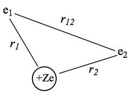
Figure 1. Model of Helium atom.

Independent Particle Model

Electron Spin

Stern-Gerlach Experiment

In 1922, Stern and Gerlach set out investigate non-zero angular momentum coupling to space. Or they asked, if the quantum number l ≠ 0, hence m_l ≠ 0 can couple to the magnetic field. They used silver atoms, which has the electron configuration of ...4d¹⁰5s¹. The experimental setup is shown in Figure 2.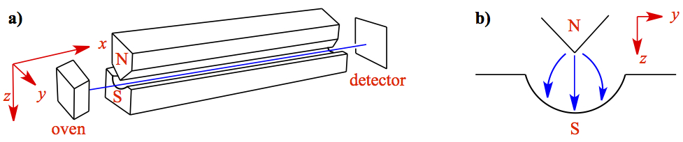
Figure 2. Stern-Gerlach Experiment. a) Configuration of set up. b) Cross section of the inhomogeneous magnetic field.

The appartus is placed in a vacuum chamber and the oven produces the collision-free beam of Ag atoms, generally referred to as molecular beam (in this case, atomic beam). You can get more information on the molecular beam in the following collapsible menu.

The magnetic moment μ of two charges separated by distance d is given as

$$\mu =q_{}d$$

1

where q is the charge of the particle. If the charges are in circular motion with angular momentum L, then the magnetic moment is written as

$$\mu =\pm \frac{q}{2m}L$$

The plus and minus sign is for the two charges. The magnetic moment in the external magnetic field gives rise to a torque on the charged particle. The force associated with a current in a wire with inifinitesimal area is given by Eqn. 6 of Chapter 1, and the force depends on the external magnetic field and magnetic dipole moment, which is equivalent to I ℓ with ℓ=length (usually it is defined as I x A x N, where N is the number of wires in a motor). So, we can write force acted on the charges in terms of magnetic dipolemoment. One can think about in a following way.

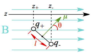
Figure x. Magnetic dipole moment in applied magnetic field

In this configuration, where the two charges rotate with respect to the mid point between the charges (ℓ/2 point), the force associated with the rotation is given as

$$F=\mu B\sin \theta$$

We can obtain the potential energy associated with magnetic dipole is

$$V=-{\displaystyle \int \mu B\sin \theta }d\theta =-\mu B\cos \theta =-\mu \cdot B$$

The potential energy of the charged particle and external magnetic field is then dependent upon both μ and B, thus,

$$V=V\left(\mu ,B\right)$$

It means that the force can be exerted to the charged particle by both μ and the magnetic field. If we consider the variation of μ in the Stern-Gerlach experiment is neglegible, the force is in the experiment is given by,

$$F={\mu }_z\frac{\partial B}{\partial z}$$

where μ_z is the z component of the magnetic dipole. The gradient of B in the z-direction gives rise to the cooupling with the magnetic dipole. The sharply triangular shape of one of the sides of the magnet used in the Stern-Gerlach experiment is due to this reason.

As we mentioned earlier, the electron configuration of the unpaired electron in silver atom is 5s¹, and since s orbital possesses zero angular momentum, we expect then the Stern-Gerlach experiment to give the following.

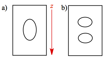
Figure x. Stern-Gerlach experiment.
a) Classical expectation, b) Result

Uhlenbeck and Goudsmit's interpretation

As it is seen, the electron in s orbital shows splitting in the magnetic field. From the orbital angular mementum, we know that there are 2ℓ + 1 components of m_l. It must mean, then, is to have 2ℓ + 1 = 2, which gives ℓ to possess magnetic quantum number of ½. Uhlenbeck and Goudsmit in 1925 explained the fractional quantum number to be electron's intrinsic angular momentum. They explain that electron is spining, hence today we call electron spin. This pictorial description must be taken as a very coarse grain of salt, as such illustration only to explain the our unease in explaining subatomic particles with our everyday experience.

Electron spin as angular momentum

Since electron spin, according to Uhlenbeck and Goudsmit, is an intrinsic angular momentum, we can expect the similar operator algebra as we found for orbital angular momentum. The two possible values of angular momenta of electron spin is assigned as either +½ or -½ with respective wave functions denoted as up spin, ↿, or α and down spin, ⇂, or β. So,

$${\widehat{m}}_s|\alpha \rangle =+\frac{\hslash }{2}|\alpha \rangle$$	$${\widehat{m}}_s|\beta \rangle =-\frac{\hslash }{2}|\beta \rangle$$	xx
$$\widehat{s}|\alpha \rangle =\frac{\hslash }{2}|\alpha \rangle$$	$$\widehat{s}|\beta \rangle =\frac{\hslash }{2}|\beta \rangle$$	xx

We can define σ as the spin function, then the z component of spin as well as the squre of s to be

$${\widehat{s}}_z\sigma =m_s\hslash \sigma$$
$${\widehat{s}}^2\sigma =s\left(s+1\right){\hslash }^2\sigma$$

where ${\widehat{s}}_z$ is the operator to project z component of spin, σ is the spin (wave) function, and m_s is the spin magnetic quantum number which assumes either ± ½. s is the spin quantum number, which is |m_s|. The operator ${\widehat{s}}^2$ is the square of the spin operator, for an electron then the eigenvalue is ¾ ℏ.

Wave function and statistics

Now that we have incorporated spin degree of freedom, we can discuss relationship between wave function and statistics, that must be dealt with before we start talking about helium wave function. In this section, we learn how collection of particles, including electrons, can be described in terms of wave function, and discuss difference between different types of particles resulting in different statistics.

Let us consider three particles distributed over three boxes. One can consider boxes to label particles and three particles with their numbering can be considered as the state of the individual particle; it is quantum number. For example, we take (1,3,2) in the following discussion to mean that the first particle is in the state with energy 1 (or instead of energy, you can think about 1 being a quantum number), and second particle is in state with energy =3, and the third particle is in state with energy = 2. We constrain the total energy to be 6, meaning that the total of its state labels adds to 6. We take all possible combinations of the individual states distributed over three positions. There are ten ways to do this, as shown below. These are distinct states, because we can see the individual boxes (positions) and individual states (quantum numbers).

Constraints:	E = 6	#of particles = 3

Group 1	(1,2,3)	(1,3,2)	(2,1,3)	(3,2,1)	(2,3,1)	(3,1,2)	1.x.1
Group 2	(1,1,4)	(1,4,1)	(4,1,1)				1.x.2
Group 3	(2,2,2)						1.x.3

In group 1, each particle possesses a different energy (or quantum number), while groups 2 and 3 possess at least two states of the equal energies. Let us now calculate the probability of randomly drawing a particle from these possibilities, and examine how the probability changes depending according to the distinguishability of particles.

Distinguishable particles

If the particles are distinguishable, meaning that we can label the particles, all of these states are distinct and measurable. If one tries to draw a particle out of the system, what is the probability of obtaining a specific particle with certain energy? The probability, P, of a given particle is a product of the probability of obtaining specific states out of each group, P_s and the probability of drawing different groups, P_g, therefore P_gs = P_gP_s. The probability of drawing group 1 state is P_g = 6/10, since there are six distinct states out of 10 total, but there is only one out of three particles that have E = 1, P_s = 1/3. Therefore, the probability of drawing a particle with energy = 1 in group 1 state, P₁₁ = P₁ P₁ = 6/10 x 1/3 = 2/10. When similar calculations are done, one obtains, P₁₁ = P₁₂ = P₁₃ = 2/10 in group 1 for a total of 6/10, P₂₁ = 2/10 and P₂₄ = 1/10 in group 2, and P₃₂ = 1/10 in group 3. When all contributions are added, the sum is equal to 1.

The number of ways a particular configuration is given can be calculated by using binomial coefficient. If we define N to be the total number of particles, and N_i to be the particles having the energy of E_i, the number of different ways to construct a particular configuration is given by

$$\left(\begin{array}{c}N\\ N_1\end{array}\right)=\frac{N!}{N_1!\left(N-N_1\right)!}$$

The total configuration can be derived to be the following. $$Q\left(N_1,N_2,\cdots \right)=N!{\displaystyle \prod _{n=1}^{\infty }\frac{d_n^{N_n}}{N_n!}}$$

+ Derivation of total configuration for distinguishable particles

The binomial coefficientfor placing N₁ particles in the bin number 1 is given in Eqn xx. The bin 1 itself has many different states for which N₁ particles have access to. Let us call those states in bin 1 as d₁. Since there are N₁ particles, there must be $d_1^{N_1}$ possible states. Therefore, the number of ways to put N₁ particles into a bin containing d₁ distinct states is given by

$$\frac{d_1^{N_1}N!}{N_1!\left(N-N_1\right)!}$$

C1

The similar derivation for bin 2, but now, there are N - N₁ particles are left, then,

$$\frac{d_2^{N_2}\left(N-N_1\right)!}{N_2!\left(N-N_1-N_2\right)!}$$

C1

and for bin 3,

$$\frac{d_3^{N_3}\left(N-N_1-N_2\right)!}{N_3!\left(N-N_1-N_2-N_3\right)!}$$

C1

and so forth. The total configuration, Q(N₁,N₂ ...), of all N_i, N_j, and etc. are given by the product of each contribution.

$$Q\left(N_1,N_2,\cdots \right)=\frac{d_n^{N_n}N!}{N_1!\left(N-N_1\right)!}\frac{d_2^{N_2}\left(N-N_1\right)!}{N_2!\left(N-N_1-N_2\right)!}\frac{d_3^{N_3}\left(N-N_1-N_2\right)!}{N_3!\left(N-N_1-N_2-N_3\right)!}\cdots$$

C1

which can be reduced to

$$Q\left(N_1,N_2,\cdots \right)=N!{\displaystyle \prod _{n=1}^{\infty }\frac{d_n^{N_n}}{N_n!}}$$

C1

Indistinguishable particles

The situation for indistinguishable particles is that we lose the ability to know where particles come from. We can only tell that for the group 1 a particle is in the state with E = 1, another particle is in a state with E = 2, and the other particle in a state with E = 3, thus P_s = ⅓ but we don't know which box the particle came from. From this point of view, we only have one state from each group; we only have three distinct states, P_g = ⅓. So, the probability of drawing a particle with E = 1 for group 1 is P_gs = P_gP_s = ⅓·⅓ = 1/9. You may exclaim that "But, we have six states in group 1!" Working with indistinguishable particles, we lose ablility to label boxes (or positions), and thus, the six possibilities in Eq. 1.x.1 must be "averaged out" in a sense of linear combination of different configurations in the group. These six possibilities are the permutation of switching the particle position (box) among the possible quantum states under the constraint of total energy equal to 6. With this line of thought, the group 1 probabilities are P₁₁ = P₁₂ = P₁₃ =1/9, while group 2 particles have P₂₁ = ⅓·⅔ = 2/9, P₂₄ = ⅓·⅓ = 1/9, and for group 3, P₃₂ = ⅓. The sum of all probabilities is again unity. Particles of this type are referred to as bosons.

It turns out that for indistinguishable particles, the number of distinct ways to place N_n particles into the d_n states in the n^th bin is

$$\left(\begin{array}{c}{N}_n+d_n-1\\ N_n\end{array}\right)=\frac{\left(N_n+d_n-1\right)!}{N_n!\left(d_n-1\right)!}$$

C1

Indistinguishable particles with further constraint, the Pauli exclusion principle

All chemists know that we are not supposed to put more than two electrons (α and β) into an orbital. The principle was born out of Pauli’s careful examination of experimental results and the periodic nature of the elements. How does this principle affect us here? Let us restate the exclusion principle by saying that no electron possesses the same set of quantum numbers. Our simple model system has three particles in three boxes that we cannot see. For simplicity, we ignore the spin quantum number. Each particle with a certain set of quantum numbers n, e.g. (3,1,2) means to have n = 3 in the first box, n =1 in the second box, and n = 2 in the third box. All particles in group 1 have different quantum numbers, Ps = 1/3, while two particles in the same quantum states are in group 2. Furthermore, three particles are in the same quantum state in group 3. Groups 2 and 3 are not valid states under Pauli exclusion principle! Thus, we only have one distinct state, Pg = 1, in group 1. Then, the probability of obtaining particle with n =1 is P11 = P12 = P13 = 1/3. As is mentioned above for bosons, the six permutations must be averaged over by a linear combination. The particles that obey the Pauli exclusion principle always possess a half-integral quantum numbers. This type of particles are called fermions.

Symmetric vs. antisymmetric functions

The physical basis of permutation came from the fact that the particles in a quantum system are indistinguishable and thus must be linearly averaged. The counting schemes we have shown above would give rise to different distribution functions in statistical mechanics. The statistics for bosons and fermions and their spins, respectively, integral and half-integral spins have been thought to be related. In non-relativistic quantum mechanics, we postulate that bosons upon exchange of two particles exhibit totally symmetric wave functions, and fermions upon exchange of two particles exhibit totally antisymmetric wave functions. These postulates have become definitively related in relativistic quantum mechanics in 1930 by Pauli.

We understand from the discussion above that for indistinguishable particles, whether they be bosons or fermions, one needs to take a linear combination to obtain, respectively, three and one distinct states in the above example. Let us look at the state represented by group 1. If we take these six in a simple linear combination to construct a wave function,

,1.x.4 where ψ_i represents each distribution in Eq. 1.x.1, and where the sum runs to six possible basis functions. The normalization constant N can be obtained from the requirement that the wave function must be square-integrable, <ψ|ψ>=1, and thus N = [n!]-1/2 with n as the number of particles. The wave function is a function of the three quantum numbers n such that ψ_i = ψ{n}. So, if we take this wave function and exchange particle positions (or boxes if you insist) of two particles 1 and 2, represented by an operator X1↔2, we get the same wave function back, . 1.x.5

This property is called permutation invariance. We can generate all six combinations by using the operators, , , and , on any starting function, such as (1,2,3). These are, 1.x.6a 1.x.6b 1.x.6c 1.x.6d 1.x.6e

The wave function possessing permutation invariance is said to be a symmetric function with respect to permutation of two particles. If, however, the total wave function has a property that, 1.x.7

The wave function is said to be antisymmetric with respect to exchange of two particles 1 and 2. It turns out that all fermion wave functions possess this property. In our example, we can construct a totally antisymmetric wave function by applying the following operators to the state (1,2,3),

, 1.x.8 where , and in order to generate two others, we need to use successive operations as we have seen above for bosons, . 1.x.9 Each time a permutation is performed, the resulting wave function gets a minus sign. Thus, we obtain a totally antisymmetric wave function, . 1.x.10 So, if we exchange particle positions 1 and 2 by using X1↔2 on the total wave function, we should obtain −Ψ. 1.x.11 Indeed, the statement above is true.

A so-called Slater determinant can be used in order to effectively construct totally antisymmetric wave functions. The Slater determinant consists of one particle wave functions with positons listed in determinantal form. Using our example, the Slater determinant is

, 1.x.12 where (n!)-1/2 is the normalization constant. The number in the parenthesis is the particle position (or which box), and the other number is the quantum number. If we expand out according to the rule for expansion of determinant (see, appendix), one obtains the same wave function as Eq. 1.x.10. Each column of the determinant represents a different quantum state (quantum number), and each row represents a different particle position (or which box the particle is in). The antisymmetric nature of the wave function, represented by Eq. 1.x.7, is manifested by interchange two rows of the determinant. Let us go back to Pauli exclusion principle. The determinant that contains two particles with the same set of quantum numbers, so that Pauli exclusion principle is violated, is given by, for example using the (1,1,2) state,

. 1.x.13 If the determinant is expanded out, one obtains (1,1,2) – (1,2,1) – (1,1,2) + (1,2,1) + (2,1,1) – (2,1,1). It gives the wave function identically equal to zero, Ψ = 0. It means then that the state of such a system does not exist, confirming the Pauli exclusion principle.

Let us summerize at this point what we have learned. The different statistics emerges from the nature of distinguishability of particles under examination. Furthermore, all quantum particles are indistinguishable particles, and in non-relativistic quantum mechanics, we state the postulates for indistinguishable particles as:

1.bosons for which permutation (or exchange) of two particles results in symmetric wave functions

2.fermions for which permutation of two particles results in antisymmetric wave functions.

For bosons, the wave function should be totally symmetric with respect to interchange of particle positions, arrived at via a simple linear combination to obtain a kind of average of the different configurations. For fermions, the additional constraint of the Pauli exclusion principle gives rise to antisymmetric wave functions upon interchange. Such wave functions can be constructed from a Slater determinant.

Excited He in 1s2s configuration

We have see that for Fermion systems, we need to antisymmetrize the wave function. We used Slater determinant to obtain the antisymmetric wavefunction of the form

$$\begin{array}{l}\Psi =\frac{1}{\sqrt{2}}\left[1s\left(1\right)\alpha \left(1\right)1s\left(2\right)\beta \left(2\right)-1s\left(1\right)\beta \left(1\right)1s\left(2\right)\alpha \left(2\right)\right]\\ \Psi =\frac{1}{\sqrt{2}}1s\left(1\right)1s\left(2\right)\left[\alpha \left(1\right)\beta \left(2\right)-\beta \left(1\right)\alpha \left(2\right)\right]\end{array}$$

Therefore, one of eitehr space or spin part of the wave function suffices for antisymmetric. In this case spin is antisymmetric to the exchange of particles.

For an excited state of helium atom with electron configuration 1s 2s, we can picture several situation as follows.

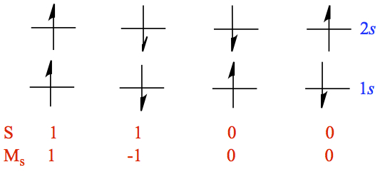
Figure x. All possible electron configurations from 1s 2s

In Figure x, the values of total spin S = s₁ + s₂ and total m_s which is denoted M_s = m_s1 + m_s2, where m_si is the value of m_s of the i^th electron. We need to have the wave function to be eigenfunctions of ${\widehat{S}}^2$ operator. If we borrow an analogy from the orbital angular momentum ℓ for which m_l runs from 0, ±1,..., ±ℓ. Here we have two states with M_s = 0.

$${\widehat{S}}^2={\left({\widehat{s}}_1+{\widehat{s}}_2\right)}^2=\left({\widehat{s}}_1+{\widehat{s}}_2\right)\left({\widehat{s}}_1+{\widehat{s}}_2\right)={\left({\widehat{s}}_1\right)}^2+{\left({\widehat{s}}_2\right)}^2+2{\widehat{s}}_1\cdot {\widehat{s}}_2$$

with

$${\widehat{s}}_1\cdot {\widehat{s}}_2={\widehat{s}}_{x1}{\widehat{s}}_{x2}+{\widehat{s}}_{y1}{\widehat{s}}_{y2}+{\widehat{s}}_{z1}{\widehat{s}}_{z2}=\frac{1}{2}\left({\widehat{s}}_{1+}{\widehat{s}}_{2-}+{\widehat{s}}_{1-}{\widehat{s}}_{2+}\right)+{\widehat{s}}_{z1}{\widehat{s}}_{z2}$$

where ${\widehat{s}}_{i-}$ is the ladder operator of i^th electron.

$${\widehat{s}}_{-}\alpha =\hslash \beta$$
$${\widehat{s}}_{+}\alpha =0$$
$${\widehat{s}}_{-}\beta =0$$
$${\widehat{s}}_{+}\beta =\hslash \beta$$
$${\widehat{s}}_z\sigma =\pm \frac{\hslash }{2}$$