Chapter 1. Thermodynamics and Classical World

Review of Thermodynamics

You should look at the following pages and understand everything about the page. The pages are the freshman chemistry material on thermodynamics.

General Chemistry Theromodynamics Chapter

Review of Newton's Law of Mechanics

1^st law: A body remains at rest or in uniform motion unless acted upon by a force
2^nd law: F = ma A body acted upon by a force moves in such a manner that the time rate of change of momentum equals the force
3^rd law: F₁ = -F₂ If two bodies exert forces on each other, these forces are equal in magnitutde and opposite direction

Energy

Total Energy is composed of kinetic (T) and potential (V) energies

T = \frac{1}{2} m v^{2}

V = V (x)

Potential is a function of position of the particle

Force, appeared in Newton's 2^nd law, can be defined as

F = - \frac{\partial V}{\partial x}

where V is the potential energy and x is the coordinate. One of chemical applications includes molecular vibration. In molecular vibration, x is given as the nuclear coordinates and V is the so-called potential energy surface with 3N - 6 (N is the number of atoms) dimensions, describing how energy change with respect to coordinates, such as bond distance, bond angle and dihedral angle, among others.

The following picture illustrates what the force is. You can think about the x axis as a reaction coordinate for which reaction proceeds from left to right. The energy change along the reaction coordinate is represented by V.

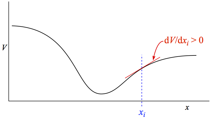
Figure 1. Relationship between potential energy and force.

As is seen in the figure, the tangent line of V at a point x_i is shown as positive slope. Therefore, the force exerted is negative of the tangent line. The force points to the negative direction. Also, steeper the tangent line, larger the force is.

+ On the potential energy curves

There are many different types of empirically derived potential energy forms available. These potential energy forms are for molecular motion or molecular vibration, thus deal with how energy changes with respect to changes in atomic positions.

Most fundamental of all is potential energy curve of diatomic molecules. Since there is only one coordinate, stretching coordinate, one can represent potential energy curve as a function of the bond stretching coordinate. Here one prominent example of diatomic molecular potential called Morse potential is given.

Morse Potential: $V (R) = D_{e} {(1 - e^{- a (R - R_{e})})}^{2}$ where D_e is the dissociation energy of a molecule, R_e is the equilibrium bond distance, and a is defined as $a = {(\frac{k_{e}}{2 D_{e}})}^{1 / 2}$ where k_e is the force constant, typically given in units such as mdyn/Å or dyn/cm, where 1 dyn = 10 μN = 10^-5 kg m / s². The force constant is related to the vibrational frequency via $ν = \frac{1}{2 π} {(\frac{k_{e}}{μ})}^{1 / 2}$ where μ is a reduced mass of the molecule, which is $μ = \frac{m_{1} m_{2}}{m_{1} + m_{2}}$ Diatomic potential energy curve looks like the following, including the important features that are in the Morse potential.

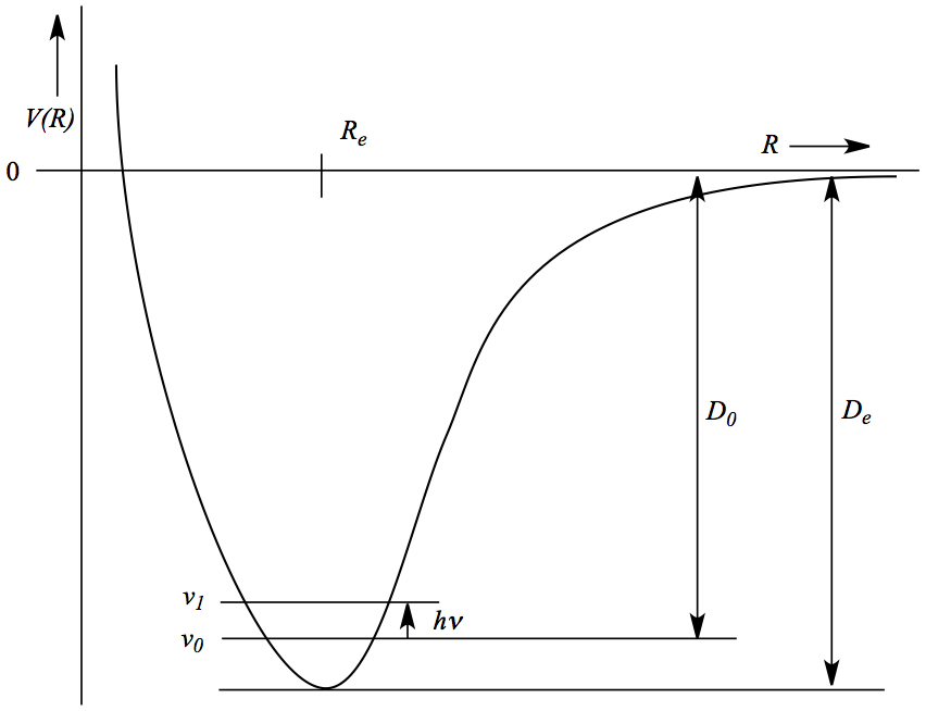
The lowest point of the potential is given by D_e, representing the dissociation energy of the molecule, and it occurs at equilibrium distance, R_e or equilibrium bond distance. Notice that the interaction energy is a negative value, indicating stability relative to the separated atoms. When the bond is stretched to the point where the interaction between two atoms are small, it is the right-hand region where the V(R) tapers down to value of 0. Zero because there is no interaction.

On the opposite side of R_e, that is to shrink the bond, compared to R_e, the intection energy goes up, eventually becomes positive number, meaning that the interacton energy is repulsive.

You can see the lines ν₀ and ν₁. These are the quantized vibrational energy levels of diatomic molecules. In order to make a transition from the lowest energy state, ν₀ to an excited state, ν₁, an infrared photon is aborbed by the molecule, which is registered in IR (or Raman) spectrometer.

The equation that relates frequency and force constant is actually an approximation equation. As long as you only look at fundamental transition, which is ν₁ ← ν₀ , the approximation is quite good.

For example, the force constant of H₂ molecule is 5.756 mdyn/Å, we can calculate vibrational frequency using above equations to be 4403 cm^-1, which is in agreement with the Raman spectra.

Brief breakdown is as follows:

5.756 mdyn/Å = 5.756 x 10² kg/s²
μ = (1.008 amu)²/(1.008 + 1.008 amu) = 0.504 amu
Using a conversion factor of 1.66053892 x 10^-27 kg = 1 amu, 0.504 amu = 0.83691 x 10^-27 kg.
ν = (1/2π)(5.756 x 10² kg/s²/0.83691 x 10^-27 kg)^1/2 = 1.3199 x 10¹⁴ /s or Hz
Using a conversion factor of 1 Hz = 3.33565 x 10^-11 cm^-1, one obtains 4403 cm^-1

Review of Electricity and Magnetism

We know that atom is made of nucleus and electrons for which they possess electrical charges, plus and minus, respectively. Absorption and emission of light, which is electromagnetic wave, is also characteristics of atoms. Therefore, understanding electricity and magnetism is quite important.

Interaction of Charged Particles

Let's start by looking at interaction of charged particles. The potential energy between charged particles i and j are denoted as V_ij, and is given by Coulomb's Law.

V_{i j} = \frac{1}{k} \frac{q_{i} q_{j}}{r_{i j}}

where q_i and q_j are the electrical charges of particle i and j, respectively, and k is a constant (k = 4πε₀ with ε₀ is called vaccuum permitivity). If q_i and q_j have the same charges, then the V is positive, indicating that the interaction is repulsive. If q_i and q_j have the opposite charges, the interaction V becomes attractive.

+ Vacuum Permittivity

The numerical value of vacuum permittivity, ε₀ = 8.854 x 10 ^-12 F/m (farad per meter) or s⁴A²m^-3kg^-1.

Farad is a unit of capacitance, a measure of capacity to hold electrical charges.

Magnetism

Magnet has two poles, north and south. A directional compus points to magnetic north pole of earth. In analogy with repulsion and attraction in electrostatics, like magnetic poles repel, and different poles attract.

In materials, there are several magnetism occurs.

Diamagnetic: Molecules of the material has all paired electrons

Paramagnetic: Molecules of the material has one or more unpaired electrons

Ferromagnetic: All unpaired electrons are lined up in one direction

Magnetic field produced by current

Classic experiment by Orsted in 1820 shows electrical current can induce magnetic field on the plane perpendicular to the wire, as shown below. Directional compasses are placed on the bench where the electrical wire is placed perpendicular direction. When a current flows through the wire, compasses point in circularly pointed.

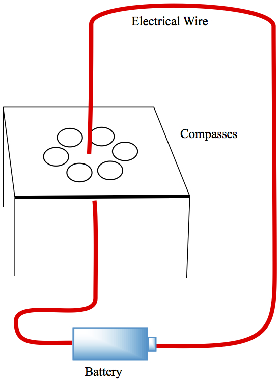
Figure 2. Magnetic field produced by electrical current

When a current is off, all compasses point to north, as usual. When, however, a current is turned on, the compasses point in circular pattern, represented by a so-called, right hand rule, as shown in Figure 3.

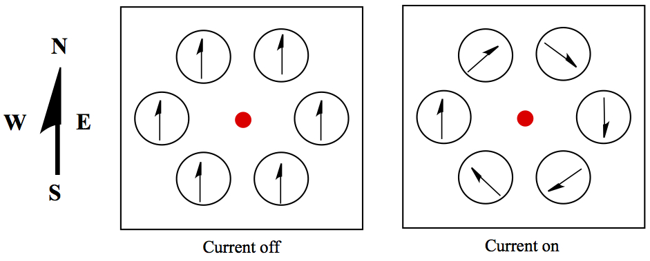
Figure 3. Result of Oersted experiment

In the above example, the right panel of Figure 3, the current is going away from the screen to the back-side of the monitor you're looking at. One can calculate magnetic field around the wire, as

B = \frac{μ_{0} I}{2 π r}

where μ₀ is vacuum permeability, I is current, and r is the distance from the wire.

+ Vacuum Permeability

The numerical value of vacuum permeability, μ₀ = 1.256 x 10^-6 NA^-2 (Newton per squared ampere) or kg m s^-2A^-2.

When the constant is combined with the vacuum permittivity, one obtains the speed of light, $c = \frac{1}{\sqrt{ϵ_{0} μ_{0}}} = 2.998 \times 10^{8} \overset{m}{} / \underset{s}{}$

Force between Two Wires

If two wires are parallel to each other and the current flows through both wires, you observe that there appears either repulsion or attraction on the wires. Using Eqn. 5, the distance r is set to the distance between wires, the force exerted on one wire is given by

F = I B l

when current is perpendicular to the magnetic field, B. The force that is feld by a segment of wire 1 carrying a current I₁

F_{1} = I_{1} l B_{2}

and we substitute Eqn 5 for B₂, we get

F = μ_{0} l \frac{I_{1} I_{2}}{2 π r}

Here, r is the distance between two wire of the length l. If the current in the two wires flow in the same direction, the force between the wires are attractive in nature, as shown in Figure 4. When the current is reversed in one wire, the force between the two wires are repulsive.

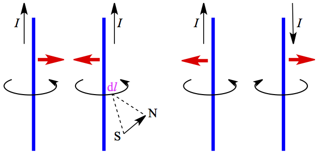
Figure 4. Force between two wires with current.

The small line segment l for magnetic field and its direction are also shown in the inset in the figure. From the orientation of these magnetic fields genearted by two wires can attest to the repulsive and attractive natures of two cases.

We can put Eqn. 5 into integral form as,

\oint B \cdot d l = μ_{0} I

The integral with a circle indicates that integration is done on the circular path that is described in Figure 4, and Eqn. 5 is a part of Maxwell's equation.

Faraday's Law of Electrical Induction

Since a current induces a magnetic field, it is possible that the opposite can happen. About 10 years after Oersted's experiment, Henry and Faraday independently examined the electrical induction effect by magnet. The following figure shouws how an experiment can be carried out.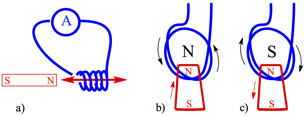

Figure 5. Current produced by moving magnet.

An electrical wire is wound up in a coil and is connected to an ampmeter, which registers the current induced by motion of a magnet. When a magnet goes through the loop of wire, the current I is induced.

The direction to which the current flow is given by Lenz Law, which states that a current will flow due to the induced magnetic field opposing the magnetic field. Use a right-hand rule, when N side of the magnet approaches the loop, as shown in Figure 5b, the induced magnetic field closer to the N side of the magnet becomes N. Thus, the magnetic field develped in the loop is counterclockwise by pointing your thumb to you, the curling of other fingers tell you the couterclockwise motion.

When the magnet is pulling away from the loop as shown in Figure 5c, then the induced magnetic field point toward the rear of the monitor you're looking at. It means that the side closest to the magnet is S. Using the right-hand rule, tell you that the current induced is clockwise. If we define magnetic flux to be the sum of magnetic line passing through an area, A, is

Φ_{B} = \int B \cdot d A

Then, the force generated to move charges to produce current, we call it electromotive force is related to electric field

E = - \frac{d Φ_{B}}{d t}

The minus sign indicates the magnetic flux is induced around the wire by the magnet, as discussed above. Then, if we consider a circular path in the small displacement dl for electric field,

Φ_{E} = \oint E \cdot d l

We can then write Faraday's law in the following form,

\oint E \cdot d l = - \frac{d Φ_{B}}{d t}

Displacement Current

A magnetic field is produced by not only by an electrical current. When a capacitor is placed in a circuit, accumulation of charges on the parallel plates should also give rise to magnetic field. Since accumulation of charge on the capacitor plates changes the electric fields,

The charge on a capacitor is given by

Q = C V

where C is capacitance and V is the potential difference between the two plates and V = Ed with E is the electric field and d is the distance between the plates. The capacitance is given by

C = ϵ_{0} \frac{A}{d}

where A is the area of each plate of the capacitor. Therefore, Q is given by

Q = ϵ_{0} A E

Then, the electric field that changes in time is given by

\frac{d Q}{d t} = ϵ_{0} A \frac{d E}{d t} = ϵ_{0} \frac{d Φ_{E}}{d t}

where Φ_E is the electric flux defined by Φ_E = EA.

Then, we can write Maxwell equation for Ampere's law to be

\oint B \cdot d l = μ_{0} (I + ϵ_{0} \frac{d Φ_{E}}{d t})

Gauss's Law

The electric flux calulated within a closed area on a surface is the net charge, Q,

\oint E \cdot d A = \frac{Q}{ϵ_{0}}

is the statement of Gauss's law. Analogous statement of Gauss's law in magnetism is given by

\oint B \cdot d A = 0

This states that the sum of magnetic flux in the area A is zero, which means that there is no magnetic equivalent of single electric charges, monopoles.

Simple Harmonic Motion

The force associated with harmonic motion is given by

F = - k x

is a linear force, also known as Hook's law. Since Newton's law of motion is F=ma, the differential equation that represents harmonic motion is

m \frac{d^{2} x}{d t^{2}} = - k x

Thus,

\frac{d^{2} x}{d t^{2}} + \frac{k}{m} x = 0

The solution to Eqn. 23 is

x = A cos (ω t + ϕ)

where A is the amplitude or the maximum displacement of mass m. The arguments of cosine function is ω is the frequency of the sinusoidal motion (or peak to peak frequency), φ is a constant phase angle to shift the wave.

Traveling Waves

Traveling wave can be represented by sinosoidal functions as we have seen above for harmonic oscillator solution. In the traveling wave case, the wave Φ(x,t) at certain coordinate x is moving with a speed v, as shown in Figure 6.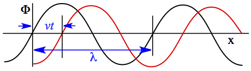

Figure 6. Traveling wave.

At some time t = 0, let's say that the wave is represented by the black curve, but when at some time has passed, the wave has shifted due to its velocity, shown as red curve in the figure. In this case, Φ(x,t) is represented by

Φ (x, t) = Φ_{0} sin [\frac{2 π}{λ} (x - v t)]

where Φ₀ is the maximum displacement of the wave amplitude, λ is the wave length and v is the velocity of the wave.

Propagation of Electromagnetic Waves

We use Eqns. 13 and 18 of Maxwell's equations to explain how electromagnetic wave propagates. Consider a small rectangular box (purple colored box) labeled with dx and dy in the electric field (wave in blue) in Figure 7.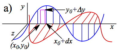

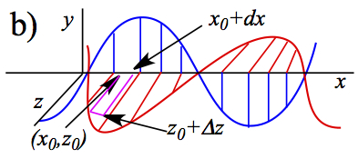Figure 7. Propagation of Electromagnetic Wave. Electric=Blue Magnetic=Red

Since the magnetic field is increasing in time in the process in the purple rectangle, the induced magnetic field in the reactangle decreases according to Lenz law, then the electric field Let us examine the propagation using Eqns. 13 and 18. The idea is to examine what's happening with the purple areas in Figure 7. In Figure 7a, the induced magnetic field in the purple loop should decrease in time with the wave moving toward +x direction. Then, the electric field should point opposite to this change. Therefore, the electric field is greater on the right side of the loop, a counterclockwise circulation (or current without electron, if you want!). The circulation produced is produced to oppose the change in Φ_B.

+ Propagation of Electromagnetic Wave

Let us assume that the solution to Maxwell's equations for electric and magnetic fields are, respectively, as follows:

$E_{y} = E_{0} sin (k x - ω t)$	c1
$B_{z} = B_{0} sin (k x - ω t)$	c2

where constant k, ω and velocity v are defined respectively as,

$k = \frac{2 π}{λ}$	c3
$ω = 2 π f$	c4
$ω λ = v$	c5

with λ is wave length and f is frequency. Eqns c1 - c5 are assumed to be the solution to the Maxwell equations, Eqn. 13 and 18, and are

$\oint E \cdot d l = - \frac{d Φ_{B}}{d t}$	13
$\oint B \cdot d l = μ_{0} (I + ϵ_{0} \frac{d Φ_{E}}{d t})$	18

The left-hand side of Eqn. 13 is

\oint E \cdot d l = (E + d E) Δ y - E Δ y = d E Δ y

Since dx is perpendicular to the electric field, E, the dx component is zero, and only contributions come from Δy. The right-hand side of Eqn. 13 is

- \frac{d Φ_{B}}{d t} = - \frac{d B}{d t} d x Δ y

is just a rewriting the definition of Phi;_B(Eqn. 10). Therefore, we have

$d E Δ y = - \frac{d B}{d t} d x Δ y$	c8
$\frac{d E}{d x} = - \frac{d B}{d t}$	c9

There is no electrical current, therefore the current term on the right-hand side of Eqn. 18 is neglected, in below. The arguments are similar to the one for Eqn. 13 and one can derive,

$\oint B \cdot d l = μ_{0} ϵ_{0} \frac{d Φ_{E}}{d t}$	c10
$\oint B \cdot d l = B Δ z - (B + d B) Δ z = - d B Δ z$	c11
$μ_{0} ϵ_{0} \frac{d Φ_{E}}{d t} = μ_{0} ϵ_{0} \frac{d E}{d t} d x Δ z$	c12
$\frac{d B}{d x} = - μ_{0} ϵ_{0} \frac{d E}{d t}$	c13

Eqn. c13 is analogous to Eqn. c9. Let us use these to obtain the value of amplitudes, E₀ and B₀ in Eqns. c1 and c2. According to Eqn. c9, taking the (partial) derivative of E with respect to x and taking the partial derivative of B with respect to t are equal to each other, i.e.,

k E_{0} cos (k x - ω t) = ω B_{0} cos (k x - ω t)

c14

Then, the ratio of E₀ and B₀ is,

\frac{E_{0}}{B_{0}} = \frac{ω}{k} = v

c15

Also, from Eqn. c13, by taking the partial derivative of B with respect to x on the left-hand side and taking the partial derivative of E with respect to time give,

$k B_{0} cos (k x - ω t) = ω μ_{0} ϵ_{0} E_{0} cos (k x - ω t)$	c16
$\frac{B_{0}}{E_{0}} = \frac{ω μ_{0} ϵ_{0}}{k} = μ_{0} ϵ_{0} v$	c17

Then, the quantities of Eqn. c16 and Eqn. c17 are the same, hence,

\frac{B_{0}}{E_{0}} = \frac{1}{v} = μ_{0} ϵ_{0} v

c18

and

v = \frac{1}{\sqrt{μ_{0} ϵ_{0}}}

c19

Therefore, the velocity of electromagnetic wave is constant.

Chapter 1. Thermodynamics and classical world view

Review of thermodynamics and background materials