We examine several systems that are analytically solvable, and gain insight into how one might solve these problems. In addition, we examine how to extend a simple one-dimensional system into multi-dimensions. Our hope is to learn about how each of the systems might have applications in chemistry.
Here is the prescription of how to solve simpler quantum problem in general.
1) Draw a model of physical system with identifying coordinates and potential energy (interaction energy).
2) Write down Hamiltonian according to the model.
3) Place Hamiltonian into Schrödinger equation.
4) Taking boundary conditions into account to solve Schrödinger equation for Ψ.
5) Solve for energy.
6) Normalize wave function.
That's it. What I'd like you to take home overall is that how the shapes of wave functions change with respect to the potential energy given, as well as spacing of quantized energy levels of a given system.
Particle in a Box
|
The particle-in-a-box system is to confine a particle in an infinitely deep potential well, as shown in Figure 1.
This is expressed as the following.
|
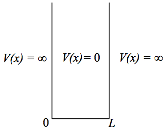 Figure 1. Particle in a box potential. |
| 4 |
| 5 |
Additionally, we want to consider the most conveniet function that vanishes at x = 0 and L. For this reason, we choose sine function as Ψ. In order to fit sine function to the interval [0,L], we use the argument of sine to be n π x / L, with n is positive integer. This way, we can fit functions such as the ones shown in Figure 2.

Figure 2. First few wave functions.
| 6 |
| 7 | |
| 8 |
Now, let us look at what the expression of energy is. As can be seen, the right-hand sides of Eqns. 5 and 8 are the same. Then, the constants assocated with them are equal, as well. That is,
| 9 |
| 10 |
Now, we need to normalize the wave function. We need to square integrate Ψ. We can follow the procedure in the section (Eqns. 8 to 11) described in Chapter 3.
| 13 |
| 14 |
| 15 | |
| 16 |
| 17 |
Figure 3 shows first three lowest energy levels and their wave functions.
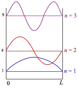
Figure 3. Energy levels and wave functions
On the left axis, the energy levels are labeled in the units of n2. The lowest energy state, n = 1 state, is called ground state. Any other states are called excited states. As the quantum number increase, the number of nodes, where the wave function becomes zero, increases.
Particle in a finite potential
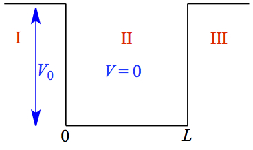 Figure 4. Finite energy well. |
In this potential, the well depth is no longer infinite. Therefore, we must consider
each of the regions (I, II, and III). Schrödinger equation for
these regions are,
|
| 20 | |
| 21 |
| 22 |
| 23 |
The first term of the right-hand side of Eqn. 21 is for region I, and the last term is for region III. It can be understood by the fact that the wave function vanish at -∞ and +∞.
We determine the coefficients on the wave functions by use of some of the conditions for well-behaved wave functions. Conditions to which the wave functions must have, are:
| 24 | |
| 25 |
| 26 | |
| 27 |
| 28 |
| 29 |
| 44 |
Particle in a 2-dimension box
Let us now extend the dimensinality of our system to 2D. It will be clear soon how to extend even to six dimensions. Let's consider the following potential.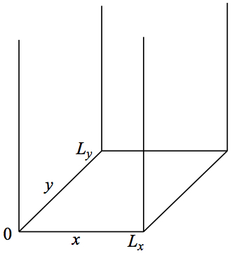
Figure 4. Particle in 2D box.
We now confine a particle in two dimensions. Similar to 1D case, we set the potential energy to be infinite outside of the box and V = 0 inside. So, we have
| 45 |
Then, inside of the box, Schrödinger equation becomes
| 46 |
Separation of Variables
The general procedure of dealing with multidimensional problem is separation of variable. In this procedure, we form the total wave function by product of one-dimensional wave functions. Thus,| 47 |
| 34 |
| 35 |
| 36 |
| 37 |
| 38 | |
| 39 |
2-D Wave functions
It means that we have separated Schrödinger equation for each dimension, for which we already know how to solve.| 40 | |
| 41 |
| 42 |
| Above is for nx = 1, ny = 1 | nx = 1, ny = 2 |
| nx = 1, ny = 3 | nx = 2, ny = 2 |
2-D Energies
The total energy of the system in 2-D is given by| 43 |
Harmonic Oscillator
So, we continue to follow the prescription of how we solve simple 1-D system. Let's make a model of the system.
Harmonic oscillator is quite important system since many things oscillates back and forth in motion. Electromagnetic wave is an obvious example, but for application to chemistry, harmonic oscillator is a model vibration. You have used IR spectrometer, a great identification instrument! Right? The energy range of IR light corresponds to the motion of nuclei in the molecule. When a carbonyl group is present, you see very prominent peak in the spectrum around 1600 cm-1, and this peak is due mainly to stretching motion of C and O in the C=O bond. We'll see later how we can obtain IR spectrum from the fundamental point of view.
In Figure 5, we have a model for harmonic oscillator and its potential.
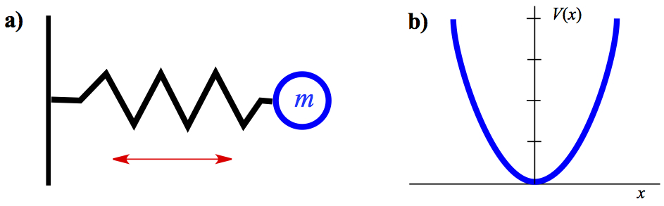
Figure 5. Harmonic Oscillator. a) Model and b) Potential.
A particle with mass m is connected to a mass-less ideal spring and move back and force in x direction. The force law comes from Hooke's law, where the force is linearly dependent on the stretching or shrinking distance.
| 44 |
| 45 |
| 46 |
| C1 | |
| C2 | |
| C3 |
| C4 | |
| C5 |
Now making the independent variable x into y by factoring out the (μω/ℏ) term.
| C6 |
| C7 |
| C8 |
| C9 |
| C10 | |
| C11 |
| C12 |
| C13 |
| C14 |
| C15 |
| C16 |
| C17 |
| C18 |
| C19 |
Now, as |y| → ∞, both the exponential part as well as the polynomial parts of Eqn. C9 become infinite, as well. In order to prevent the unphysical infinity, we limit the terms of the polynomial expansion. This can be achieved by recurrsion to stop in Eqn. C19. It means that if D in Eqn. C19 is 2n + 1, then an+2 = 0. From the definition of D, we have
| C20 |
| C21 |
| C22 | |
| C23 |
| C24 | |
| C25 |
| C26 |
| C27 |
We make some substitution and change variables.
| 47 | |
| 48 | |
| 49 |
| 50 |
| 51 |
| 52 |
The normalization procedure is the same, except the fact that it is bit more involved. So, its derivation is skipped. The normalized wave function is
| 53 |
The first few Hermite polynomial is listed in Table 1.
| n | Hn(y) | En | Normalized Wave Function |
|---|---|---|---|
| 0 | 1 | ||
| 1 | 2y | ||
| 2 | 4y2 - 2 | ||
| 3 | 8y3 - 12y | ||
| 4 | 16y4 -48y2 + 12 | ||
| 5 | 32x5 - 160y3 + 120y | ||
| 6 | 64x6 - 480y4 + 720y2 - 120 |
One of the most interesting aspect of the quantum mechanical solution to the harmonic oscillator model is that there is a n = 0 is quantized to be higher than the bottom of the well. This is what we call zero-point energy. So, the loweest possible energy seen in the potential can not be achieved by quantum systems! Quite intriguing! Also, you might have already noticed, but the energy spacing between two adjacent energy levels are the same. Look at the En column of Table 1. Each and every adjacent energy levels have hν.
Classical turning point
As has been mentioned that when a ball is placed in a 1-D bowl (consider that there is no friction), and you let go. You can easily guess the motion of the ball goes back and forth. The point at which the ball stops moving and the momentum changes its direction, is what we call classical turning point. That's exactly what we expect, say, you stretch a spring and let go. It will bounce back to original stretched length, but not beyond. You can see that in Figure 6.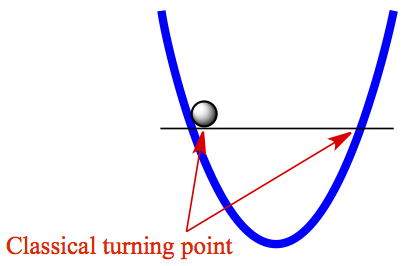
Figure 6. Classical turning point on harmonic oscillator.
Now, look at our wave function. Let us plot the ground state wave function along with its energy and the potential energy function. It is shown in Figure 7. The potential energy function represented here has mass, μ, and force constant, k, are set to 1 in Eqns. 34 - 36.
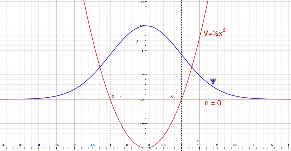
Figure 7. Harmonic oscillator zero-point energy and wave function.
In the figure, the lowest energy state (zero-point energy), red line labeled with n = 0, is superimposed on the potential energy curve (red). The blue curve is the ground state wave function. The dashed vertical lines represent the position of x = 1 and -1. The classical turning points occur at these points. Now, you might have noticed already, but the where the dashed lines meet the wave function, the value of the wave function is not zero. In fact, there are finite probability exists beyond the classical turning points. Figure 8 shows the classically allowed region is shaded for the probability distribution, | ψ |2.
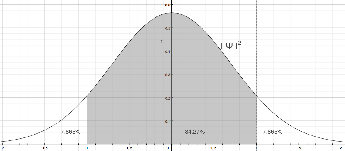
Figure 8. Classically allowed region of ground state harmonic oscillator
Since we measure the probability of finding a particle is normalized to be one we can think about how much of that particle, in a probablistic sense, can be found in the classical region vs. outside of classical realm; let's call it tunneling region. The classically allowed region is nearly 85%, while the two extreme ends have about 15% together! So, 15 out of 100 oscillators might be found outside of what is expected! That's odd!
The region outside of classically allowed one is generally referred to as tunneling. There is a bunch of examples of tunneling in chemistry. I'll show you some little later.
Harmonic oscillator as molecular vibration
As mentioned briefly above, harmonic oscillator model is used to gain information on molecular vibration.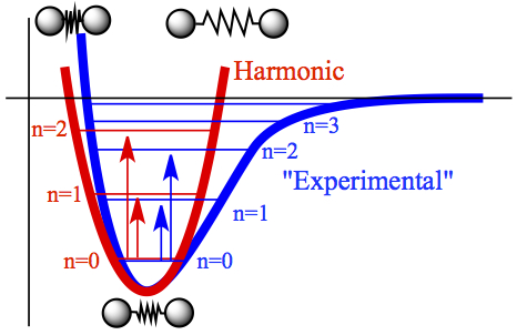
Figure 9. Energy levels of harmonic oscillator and "Experimental" potential.
One can think about a diatomic molecule to be two balls hooked up with a spring, as shown in Figure 9. The red curve is the potential energy in harmonic oscillator model, with its quantized energy levels and the transition between n = 0 state to higher states. Similarly, in blue, the potential energy obtained from experiment is given. Also shown are the energy levels according to the experiment and the transitions from n = 0 to higher states. The energy spacing for harmonic oscillator model is, of course, constant given by hν, while for the blue curve, the energy spacing between adjacent levels gets closer as energy becomes higher. Despite the fact that overall shapes of the two curves are different, in the vicinity of the lowest energy points, the two curve match decently. So, only near the equilibrium bond length, harmonic oscillator model for vibration is valid. What I mean by "valid" is that the fundamental transition, that is the molecule in the n = 0 state absorbing a photon to become n = 1 state, a primary transition registered by an IR spectrometer as a peak in the spectrum, is good enough as an approximation to molecular vibration. As it can be seen in the figure, the fundamental transition for the blue curve closely matches with that of the red potential. This is not the case for higher transition, n = 0 to n = 2, for example.
This is the general shape for stretching of any chemical bond from the small bond distance to large and eventually dissociates into two atoms. At a very large distance, two atoms don't interact, therefore, the potential energy curve tapers off to asymptotic value, which can be made to be zero. The details are much rather complicated because by stretching one coordinate, other parts of the molecule is affected, and the fact changes among other things, dissociation energy and the force constant associated with the particular stretching coordinate.
Generally, what we do in the theoretical calculations to obtain the molecular geometry at equilibrium bond distance, then calculate what is known as Hessian which is the second derivative matrix of the molecular energy with respect to all coordinate. One way to think about what Hessian is, is from your undergrad calculus class. At extremum, second derivative tells you whether the function in question is concaving up or down. Right? So, the second derivative characterizes the concavity of the function at the extremum.
Also, let me approximate the potential energy curve by Talor series expansion. What I'm trying to do here is that you only have the knowledge of the bottom of the well geometry. Now you have to "feel" around the bottom of the well by moving your atoms ever so slightly in two directions, back and forth. The Taylor series expansion of the potential is,
| 54 |
| 55 |
For molecules beyond diatomic molecules, we need to transform the Cartesian coordinate to normal coordinate, which is a way to separate coordinates that are strongly bonded together, oscillating atoms are unisome and having the same frequency. Since each atom can move in x, y and z diredtion and contributing to the vibration, which means that there are 3N different frequencies are available with N being the number of atoms in a molecule. It turns out that three of 3N coordinates are taken as translational motion, and another three coordinates are for rotation for non linear molecules. The rest of the coordinates, 3N - 6 of them, are for vibrational degrees of freedom. For linear molecules, two of the rotations are equivalent, so the number of vibration becomes 3N - 5.
The normal mode analysis gives the vibrational frequencies of a molecule and for each frequency how each atom moves. The coordinate to which the atoms move in one frequency is called normal mode.
For a molecule with more than two atoms, it is not obvious how molecule vibrates. For a diatomic molecule, there is only one coordinate for which the distance between two atoms either shrink or elongate. What happens to a molecule such as water? How does it vibrate?
This is what normal mode analysis gives. The normal mode analysis is valid only in the local region of much larger global potential energy surface. It makes sense to limit to the small region. Afterall, when the IR spectrosopy is carried out, the spectra obtained are generally in the vicinity of the minimum that the molecule was in.
The model of a molecule is a linear triatomic molecule to make the argument simpler, as shown in Figure C1.
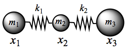
Figure C1. Linear triatomic molecules.
When the molecule vibrates, the coordinates, x1, x2, and x3, assiciated with each mass change in time. Since the motion is assumed to be harmonic (oscillatory), we can write the motion in terms of displacement xi, where i = 1, 2, and 3, from the equilibrium in the following way.
| C1 |
| C2 |
| C3 | |
| C4 | |
| C5 |
If you think what is just written is rather arbitrary, then you should consider setting up Lagrangian function, L,, which is used in dynamics often. It is set up such that L(q, ,t) = T(q, , t) - V(q), with , where is the time derivative of q. Then, solve the following equation.
| C6 |
Now we seek a new coordinate by transforming these relationships such that all masses vibrate with the same frequency ω. We can substitute Eqns. C1 and C2 into Eqns. C3, C4, and C5, then we divide each equation by eiωt. Then, we get
| C7 |
| C8 |
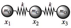
Figure C2. CO2 molecule in stretching coordinates.
So, the matrix equation C7 becomes
| C9 |
| C10 |
| C11 | |
| C12 | |
| C13 | |
| C14 |
ω2 = 0 case.: Substituting ω2 to Eqn. C9, we get from first row, A1 = A2, and the third row similarly has A2 = A3. These are substituted into the second row, we get zero. Therefore, there is no relative motion. This is a translational motion.
ω2 = k/mO: Substitution gives A2 = 0 from the first and the third row. It means that A1 = -A3, as shown in Figure C3.
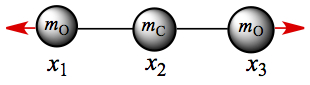
Figure C3. CO2 normal mode: Symmetric stretch.
ω2 = 2k/mC + k/mO: Substitution gives A1 = A3 from the first and third rows. The second row gives A2 = -2A1 mO/mC. So, the two oxygen atoms move in the same direction and the carbon atom moves in one direction, as shown in Figure C4.
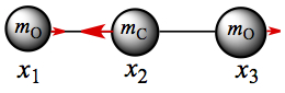
Figure C4. CO2 normal mode: Asymmetric stretch.
For a general case, we can see from Eqn. C7 that diagonal terms contain mass and frequency2 product with force constant, while off-diagonal elements are the negative of force constants, which shows connectivity of atoms in a molecule.
Rotations
Next model system we're going to examine is rotations. This leads to discussion of how the shapes of atomic orbitals are the way they are, and this has to do with the angular momentum of the electron in the atom. Let us start with a simpler example of a particle on a ring system.
Classically, rotational kinetic energy is described by angular momentum. For a mass m to travel around a circle with its radius r, we can see that circumference is given by
| 56 |
| 57 |
Angular momentum give a force perpendicular to the plane of rotation, as shown in Figure 10. This is the same force acting on the wheels of bicycle, and when the speed is too high, it is hard to turn.
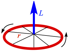
Figure 10. Angular momentum of a wheel
Hamiltonian in 3-D rotation
Before moving to relatively simple system of particle on a ring, I'd like to show how Hamiltonian looks like in all full 3-D rotation. Let me give you a new coordinate system, a spherical polar coordinate. The coordinate in relation to Cartesian system is shown in Figure 11.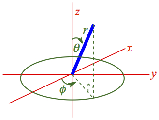
Figure 11. Spherical coordinate system |
The mass is attached at the end of line segment r. The coordinate system along with Cartesian coordinates are in Figure 11. The angle φ is the polar angle formed by the projection of r on the x-y plane. It starts on the positive x axis in counterclockwise fashon. The angle θ is the azimuth angle of the r to the z axis. |
The Hamiltonian of 3-D rotation in spherical polar coordinate is written as the following.
| 58 |
It looks rather formidable.
Particle on a ring
Let us look at a simpler system, where the rotation only occurs on a ring with a fixed r. It means that we need to fix θ = π/2 (which makes sinθ = 1), and ∂/∂θ goes to zero, because it is not changing. Then, we have much more benign looking Hamiltonian,| 59 | |
| or | |
| 60 |
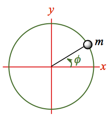
Figure 12. Particle on a ring system
Now place Hamiltonian (Eqn. 60) in Schrödinger equation, we have
| 61 | |
| 62 |
Boundary condition
The boundary condition for this system is called cyclic boundary condition in that the function Φ must have the same value after one revolution. It means that Φ(φ) = Φ(φ+2π). Figure 13 shows the cyclic boudary condition, where Φ(0) = Φ(2π) with the matching first derivatives, as well.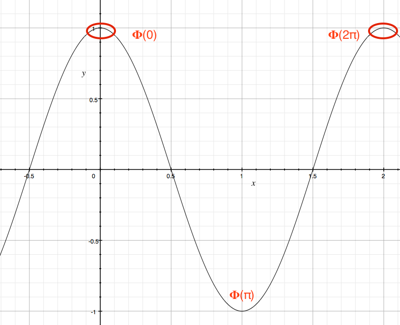
Figure 13. Φ = eimφ at φ = 0 and 2π
Normalization
So, we assume the wave function to have the form,| 63 |
| 64 | |
| 65 | |
| 66 |
Energy
By differenciating the wavefunction twice, you get| 67 | |
| 68 |
| 69 |
| 70 |
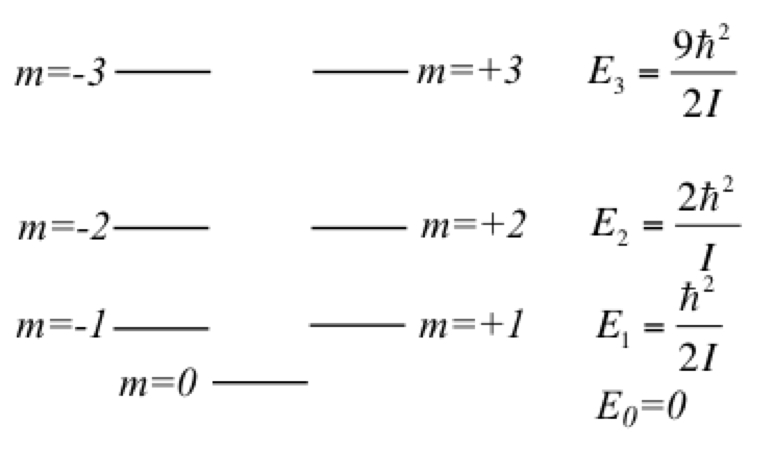
Figure 14. Energy levels of particle on a ring
The wave function and density for the lowest three sets are given in Figure 15. For m = 0, the amplitude is constant. For higher energy states, the number of nodes increase by two as the absolute value of m increases by one to meet the cyclic boundary condition requirement.
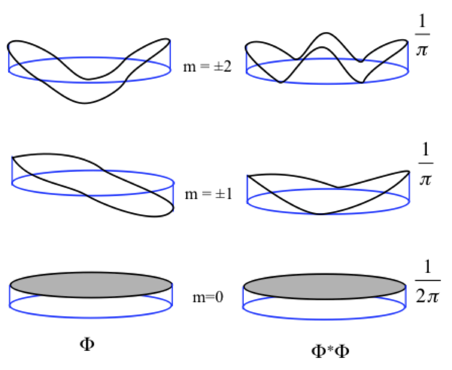
Figure 15. Wave functions of particle on a ring
Here is a cute illustrative example using particle on a ring system.
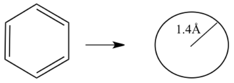
Figure E1. Benzene as particles on a ring system
Since there are six electrons in π-orbitals, three lowest orbitals should be occupied. The transition for absorption of the longest wave length is from HOMO-LUMO. If we consider HOMO of benzene to be E±1 and LUMO to be E±2 states, the hν = E2 - E1. In atomic units, electron mass me = ℏ = 1, and c = 137.036. Using these we have,
| E1 |
| E2 |
| E3 |
| E4 |
The observed wave length is 255 nm for benzene. In ball park, not too bad for a back-of-envelope.
Particle on a sphere
Now we're expanding the system from rotation on a plane to rotation on a sphere. However, again, we limit ouselves to have a constant radius, or rigid rotor approximation. Since r is constant, its derivatives are all zero in Eqn. 58. Furthermore, we consider free rotor, which means V = 0 on the sphere. Therefore, Hamiltonian for the system becomes| 71 |
Separation of variables
In Eqn. 71, we have two variables, θ and φ. We need to separate variables such that we have Schrödinger equation for each variable. We form the total wave function, denoted as Y, in the product form, as we have seen few times when two or more variables are involved| 72 |
| 73 | |
| 74 |
| 75 |
The left-hand side is much harder! We set the left-hand side a constant.
| 76 |
| 77 |
| C1 |
| C2 |
| C3 |
| l | Pl(x) |
|---|---|
| 0 | P0(x) = 1 |
| 1 | P1(x) = x |
| 2 | P2(x) = (3x2 - 1)/2 |
| 3 | P3(x) = (5x3 - 3x)/2 |
| 4 | P4(x) = (35x4 - 30x2 + 3)/8 |
| 5 | P5(x) = (63x5 - 70x3 + 15x)/8 |
When m ≠ 0, then we need to seek full solution to Eqn. C1. The solution to Eqn. C1 then is called associated Legendre polynomial,
| C4 |
| l | m | Pl(x) | Pl(cosθ) |
|---|---|---|---|
| 0 | 0 | P0(x) = 1 | = 1 |
| 1 | 0 | = x | |
| 1 | 1 | = (1 - x3)1/2 | |
| 2 | 0 | = (3x2 - 1)/2 | |
| 2 | 1 | = 3x(1 - x2)1/2 | |
| 2 | 2 | = 3(1 - x2) | |
| 3 | 0 | = (5x3 - 3x)/2 | |
| 3 | 1 | = 3(5x2 - 1)(1 - x2)1/2/2 | |
| 3 | 2 | = 15x(1 - x2) | |
| 3 | 3 | = 15(1 - x2)3/2 |
Put together the whole thing, 3D rotation
Now, let's look at them as a whole. First, the wave function is Θ·Φ called spherical harmonics, Y(θ,φ), and has a form,| 78 |
Hydrogen Atom
Hydrogen atom is an extension 3D rotation, except that we need to to let go of restriction of constant r, and we have attractive potential Read the section of hydrogen atom in Lowe and Peterson! Sorry, I was not able to finish this section up!!